“Getting a solubility value using minimum amount of compound provides a lot of value. Especially when the compound is very hard to synthesize.”

Organic Chemist
If we are to create a wish list for solubility measurement, what would it be? The ideal solubility measurement should be rapid, sensitive and using minimum amount of compounds. It must have a wide application coverage (different samples, solvents, pH, temperatures, excipients) and should deliver reproducible results. Preferably, the full process from sample preparation to measurement and analysis is fully automated to minimize errors and decrease hands-on time.
Is this possible? It is now. How? Using The Solvent Redistribution Method from Oryl Photonics.
The Solvent Redistribution (SR) method detects the solubility and aggregation of compounds by measuring how the solvent redistributes around the solute molecules as they transition from monomeric state to aggregated state (dimers, trimers, etc) as shown in Figure 1. The SR method detects the onset of aggregation at concentrations below the range where turbidity occurs. It is thus more sensitive than turbidity measurements while retaining the advantage of speed. Additionally, it is precise with exceptional reproducibility. Visit this page for a detailed benchmarking study.
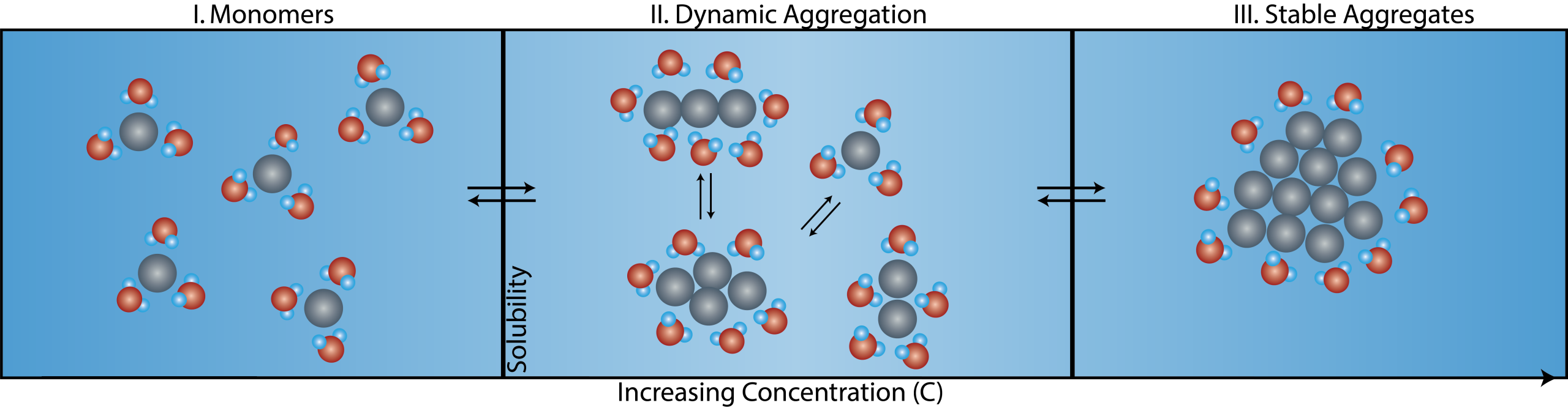
Figure 1: Schematic of aggregation for the Solvent Redistribution method. With increasing solute concentration, solute monomers transition to stable aggregates. In-between fully dissolved monomers and stable aggregates, there is a concentration range where different types of structures (dimers, trimers, etc.) co-exist. The distribution of solvent molecules around these structures change dynamically – hence the term Solvent Redistribution. Relative to the monomer state, there is an increase in the number of solvent molecules around the solute at the onset of aggregation that can be used a metric to detect the solubility limit.
Figure 1 shows the figure of concept for the SR method. With increasing concentration, the solute transitions from monomers to stable aggregates. Within the transition phase, there exists a dynamic phase of different types of structures (dimers, trimer, quadrimers, etc.) that is characterized by a higher degree of structural anisotropy. Correspondingly, the solvent around these structures redistributes and fluctuates, hence the term Solvent Redistribution. The Solvent Redistribution method is based on high-efficiency second harmonic (SH) scattering that directly measure the interfacial solvent redistributions. At the onset of aggregation (nucleation), there is an increase in the number of interfacial solvent molecules that leads to a steep increase in the SH intensity – this is used as a metric to measure the solubility limit.
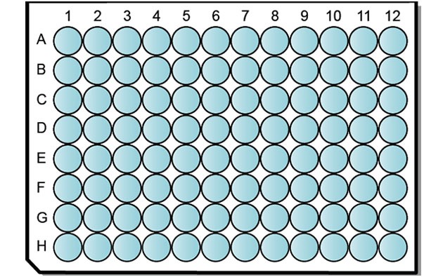
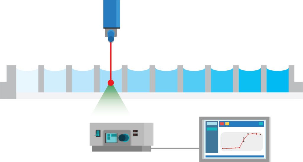
Our solubility measurement service workflow typically uses Echo Acoustic robot to directly transfer stock solutions using 10 mM DMSO stock solution. We then add the target solvent and incubate for 3 hours in a plate shaker before we screen the well-plates with Oryl’s proprietary instrument.
Key Features:
When to Use
How It Works
Fully automated solubility measurement process. The full process of solubility measurement is automated with liquid handling robots and Oryl’s instrument.
More information here:
Rapid and sensitive solubility measurement with minimum quantity of compounds | ORYL Photonics
For high-throughput measurements, you can plate the compounds directly using your in-house ECHO acoustic robot and ship them to us, properly sealed. We then add the target solvent and incubate for 3 hours in a plate shaker before we screen the well-plates with Oryl’s proprietary instrument.
Key Features:
When to Use
How It Works
Storing compounds that already aggregate in DMSO is a waste of time and energy. You can avoid this. We can perform non-destructive quality control (YES/NO, presence or absence of aggregates) of your compound libraries. Simply ship to us the well-plates where you store your compound libraries, properly sealed. We will test them in our instrument, provide you with a report and ship the well-plates back to you. You will get a YES (green) / NO (red) aggregation characterization for each compound.
Key Features:
When to Use
How It Works
The process begins with defining your experiment details in our user-friendly, web-based experiment configurator. You can specify key elements such as:
Once you finished the experimental setup:
Please review Oryl Photonics General Terms and Conditions (GT&C) before you send your chemicals. We don’t need to know the structure of your compounds. We only need to know in advance any potential hazards or dangers associated with handling, testing, storing and disposing of the compounds.
After we receive your compounds, we will perform the experiment using the protocol that we both agree. We use Oryl’s proprietary instrument that provides two orthogonal measurements: our proprietary second harmonic scattering together with ultra-sensitive linear scattering. This stage includes:
Quality Assurance
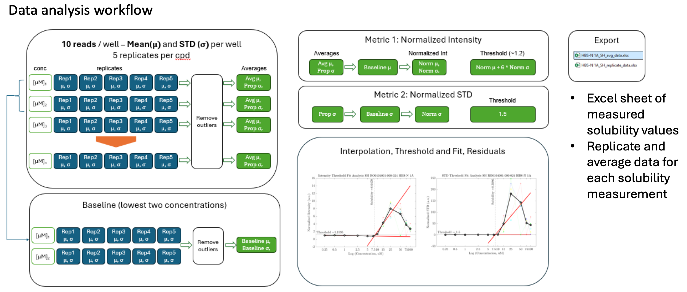
Once the measurement is complete, the results undergo automated and rigorous analysis. Our data analysis workflow (see below), automatically analyses the measurement, removes outliers and generate reports of measured solubility graphs and a spreadsheet summary of measured solubility values and readout (intensity and standard deviation).
At Oryl Photonics, we developed a technology based on Second Harmonic Scattering (SHS). This is the combination of second harmonic generation and light scattering.
Second harmonic generation is an optical process where light at a fixed frequency illuminates and excites a material following specific rules. The light and the matter interact, and the material will re-emit the light at twice the frequency of the original (incident) light. This light at twice the frequency is called second harmonic light. This means for instance that when the incident light has a wavelength of 1030 nm (near-infrared), the emitted second harmonic light will have a wavelength of 515 nm (green).
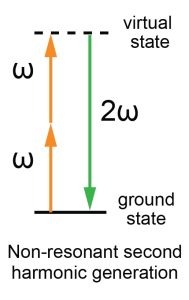
Energy diagram of non-resonant second harmonic generation: Two incident photons at frequency ω excite the material to a virtual state. The material then emits a new photon at frequency 2ω – the second harmonic – and relaxes to its original ground state.
As this optical process changes the wavelength of the light during the interaction (2 photons combine into one), it is called a non-linear process. On the opposite, the process where the wavelength would remain the same (one photon converts into one photon) is defined as linear.
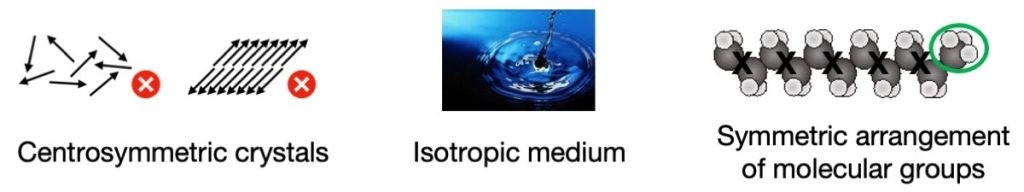
This non-linear process occurs when specific conditions are met within the material. In general, when there are centrosymmetries (symmetries around a point), there are destructive interferences, and second harmonic is not generated.
Only when both of these conditions are met, second harmonic is generated by the material under illumination. For example, there is no second harmonic generated in the following cases:
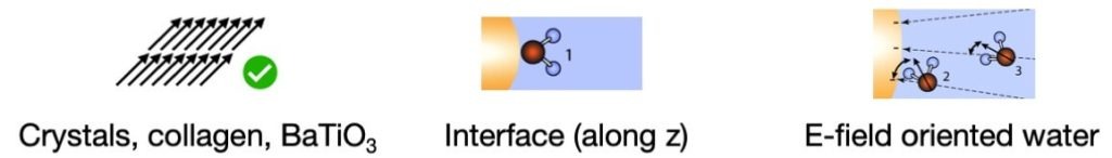
On the opposite, second harmonic generation is allowed in these cases:
Because of this peculiar symmetry dependance, studying the second harmonic light emitted by a material provides a wealth of information on how its molecules are structured.
There are several ways to implement it. The first one is to shine your laser light on a planar sample and look at the second harmonic light that is reflected by the surface. the problem is that such surface studies are very sensitive to impurities, thus the samples are challenging to prepare. Also, these interfaces do not represent well the real interfaces in nature, where real flatness is scarce.
The solution is to combine second harmonic generation with a scattering geometry. When shining the laser through the sample, second harmonic light will be generated in different directions. By collecting this scattering, you can probe the bulk of the material and you are not restrained to flat surfaces. The preparation of samples is less tedious and you can study more complex and realistic systems similar to what you find in nature. Second harmonic scattering is especially suitable to probe bulk media such as liquids, or particles, vesicles and droplets in suspension where there is no planar interface. It is used to study liposomes, emulsions, or even pure liquids.
One key application is the measurement of solubility: when a drug compound is not dissolved properly in a liquid, undissolved particles float in the liquid. This is an interface between the particle and the liquid molecules around it. The molecules reorient and redistribute to accommodate the presence of the particle, on a large volume. Second harmonic scattering can then probe the rearrangement of the liquid, the solvent, in a very sensitive way. This is what we call the Solvent Redistribution method.
Technical
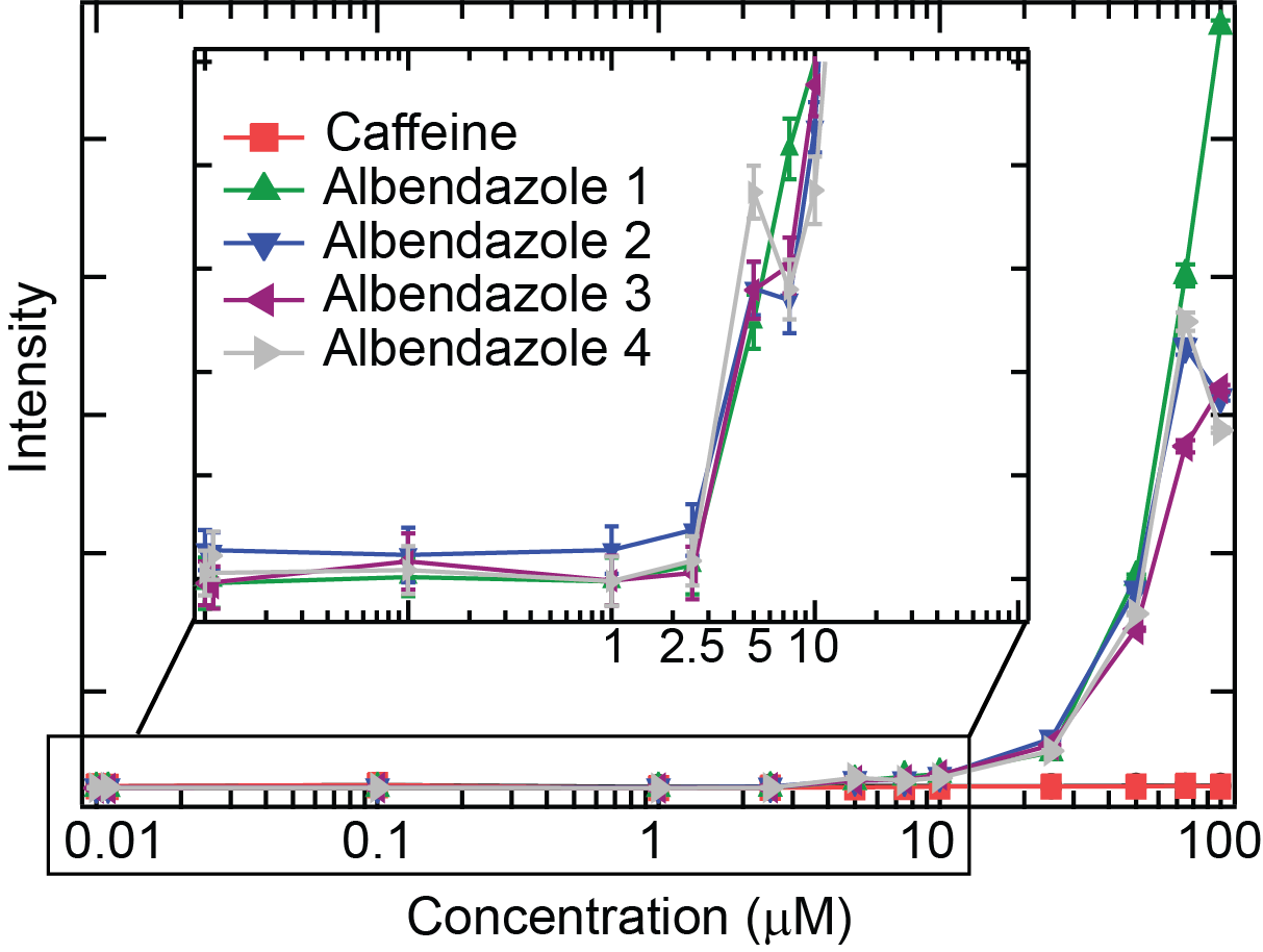
The typical output for a solubility measurement is a plot of intensity vs concentration. For example, the figure below shows the intensity vs concentration plot for a poorly soluble compound, albendazole with n=4 replicates. A control plot of intensity vs concentration is also shown for caffeine that is soluble in the range of concentrations tested.
At concentrations below the solubility limit (<2.5 µM), the intensity is low and constant (which defines the baseline). At concentrations above the solubility limit, the intensity increases. For albendazole, the intensity starts to increase from 1 µM and a clear jump in intensity is visible at concentration above 2.5 µM. For comparison, the intensity of caffeine stays flat, which indicates that caffeine is soluble within this range of concentrations.
A typical measurement report will contain a tabulated summary of the approximate solubility values for each compound, a detailed plot and solubility analysis for each compound, the protocol used for the solubility measurement and a brief explanation of the solvent redistribution method. Additional analysis can be performed on request.
The Solvent Redistribution method is a general and flexible method that looks at how the solvent redistributes as the solute transitions to different stages of aggregation. The method can be performed at different pH, temperature, pressure, salt concentration, etc.
Typical negative control is caffeine (very soluble compound) and typical positive controls are amiodarone and albendazole (poorly soluble > 1 µM).
The Solvent Redistribution method is based on high efficiency second harmonic light scattering (SHS) that probes the anisotropic distribution of solvent molecules (dipolar molecules such as water, DMSO, methanol, etc) around solutes. This unique structural sensitivity makes SHS sensitive to aggregation.
“Getting a solubility value using minimum amount of compound provides a lot of value. Especially when the compound is very hard to synthesize.”
“After using the Oryl Screener, it is hard for me to get back to the traditional techniques. It’s just too laborious.”